Deep Unfolded Robust PCA

The world is low rank + sparse

A huge class of real datasets is the superposition of a structured low rank part, a few sparse outliers, and some dense noise. The job is to pull those pieces apart.

A security camera, in one matrix

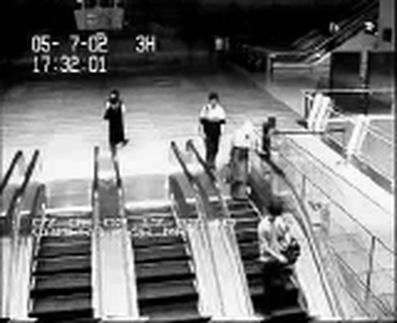
Stack every video frame as a column of a matrix D. The unchanging background repeats across columns, so it is low rank L. The people walking through appear in a few pixels of a few frames, so they are sparse S.

background = low rank L people = sparse S sensor noise = N

The classical tool: Robust PCA

Robust PCA already solves this beautifully, by convex optimization. But it has two practical pains that deep unfolding is built to fix.

The system model

We observe one matrix D ∈ ℝn×n that is the sum of three components, and we want to recover the first two.

From rank & count to a convex problem

"Low rank" and "few nonzeros" are non convex and intractable. We relax them to their convex surrogates: the nuclear norm ‖·‖* (sum of singular values) and the ℓ₁ norm ‖·‖1.

Convex, but with two non smooth terms exactly what proximal gradient is made for.

One iteration = gradient step + two proximal shrinks

Take a shared gradient step on the data fit term, then apply the proximal operator of each prior. Repeat ~200 times.

Three scalars drive everything: step size α and the two shrink thresholds τL, τS. Hold that thought.

Unroll the solver into a network

Take K iterations and treat each one as a layer. The fixed scalars become learnable per layer parameters (αk, τLk, τSk), trained end to end by backprop.

10 learned layers stand in for ~200 hand tuned iterations. Positivity of the parameters is enforced with softplus.

Structure from the model, knobs from the data

This is the heart of model based deep learning: not a black box net, and not a hand tuned solver, but the best of both.

How we test it

Train on synthetic D = L + S + N matrices with known ground truth, then compare three methods on held out data with a fixed seed.

10 layers ≈ 200 iterations, at 18× the speed

Main setting n=32, rank=4, 5% sparsity, σ=0.05. Truncated SVD recovers L but cannot separate outliers (S error 0.57), confirming explicit sparsity modeling is essential. The model based DL win: a fraction of the compute for almost the same accuracy.

Where it wins, and where it doesn't

Holding the model fixed (K=10, same budget) and varying only the rank deconfounds capacity from rank. The honest picture:

rank	method	L err	S err	F1
4	Classical	0.135	0.183	0.995
4	Unfolded	0.155	0.202	0.984
6	Classical	0.138	0.233	0.986
6	Unfolded	0.201	0.217	0.971
8	Classical	0.150	0.305	0.960
8	Unfolded	0.233	0.289	0.933

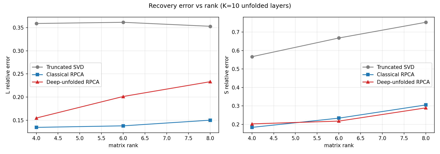
Classical wins on low rank L at every rank and the gap widens (1.15× → 1.55×): 10 layers can't resolve a higher rank subspace like 200 iterations can. But unfolded overtakes on sparse S at rank 6 & 8, and stays ~18× faster. Training had converged, so this is a capacity ceiling.

Capacity ≈ iteration budget: depth closes the gap

If the L gap is a depth ceiling, deeper should close it. At K=12 the unfolded net beats classical on both components, even at rank 8.

↓ 40%

L error vs classical at rank 8 (0.092 vs 0.150)

↓ 50%

S error vs classical at rank 8 (0.150 vs 0.302) and still ~15× faster

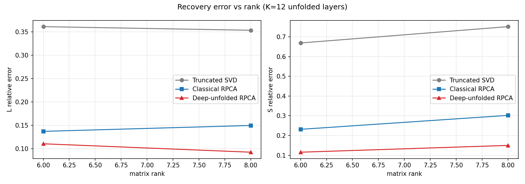
One layer ≈ one iteration of capacity. Match depth to difficulty and unfolding wins outright, an order of magnitude faster.

From synthetic training to a real security camera

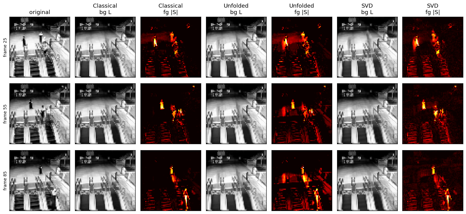
We trained only on synthetic video shaped matrices, then froze the model and ran it on a real escalator clip it had never seen. Below, the same clip is decomposed by the classical solver and by our network, side by side.

Three methods, side by side

Our unfolded background is indistinguishable from classical, and its foreground catches the moving people (a touch brighter and more permissive). Truncated SVD separates them the least cleanly. The same answer as the slow solver, an order of magnitude faster.

What we'd be honest about